Question
Mathematically speaking, holds true in Fig-1, so there is a common inference that A and B are same. But the distance itself actually means both A and B have same amount of numeric changes relative to O, without indicating the direction of the change. This is in particular a problem what if and are two genes driving different biological processes, or two factors suggesting distinct customer preferences.
There is a gap between the numeric difference (or similarity) and identity difference (or similarity).
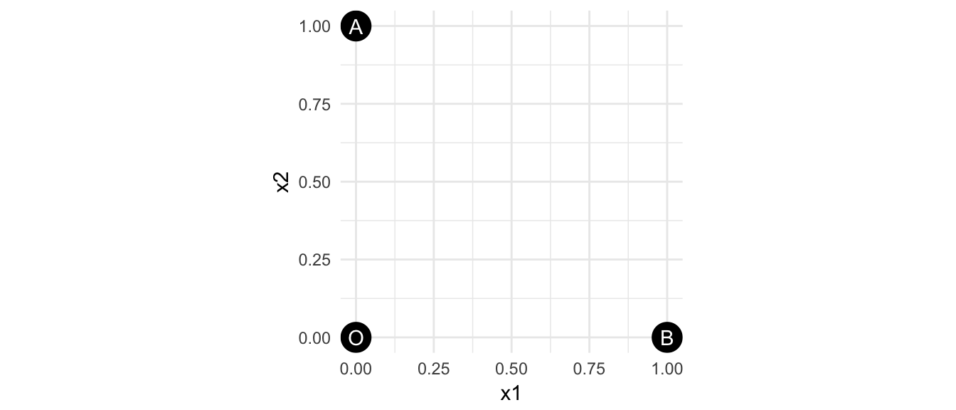
Figure 1: Are A and B same?
Further Motivation
Goal
Arbitrarily make up cell-type “O”, “A”, “B” such that “A” and “B” generally have same shifts from “O”. And to see how distance-based method decides whether “A” and “B” are the same types.
Create “O”
Suppose there are genes in total with three categories of the low (1-10), medium (100-200) and high (800-1000) expressed genes. Each cagegory has 150 genes. The general expression profile is nothing but a vector .
num_genes <- 450
expect_apple <- round(c(
# low
runif(n = num_genes/3, min = 1, max=10),
# medium
runif(n = num_genes/3, min = 100, max=500),
# high
runif(n = num_genes/3, min = 800, max=1000)
))
idx_low <- 1:num_genes/3
idx_med <- (num_genes/3 + 1) : (num_genes/3*2)
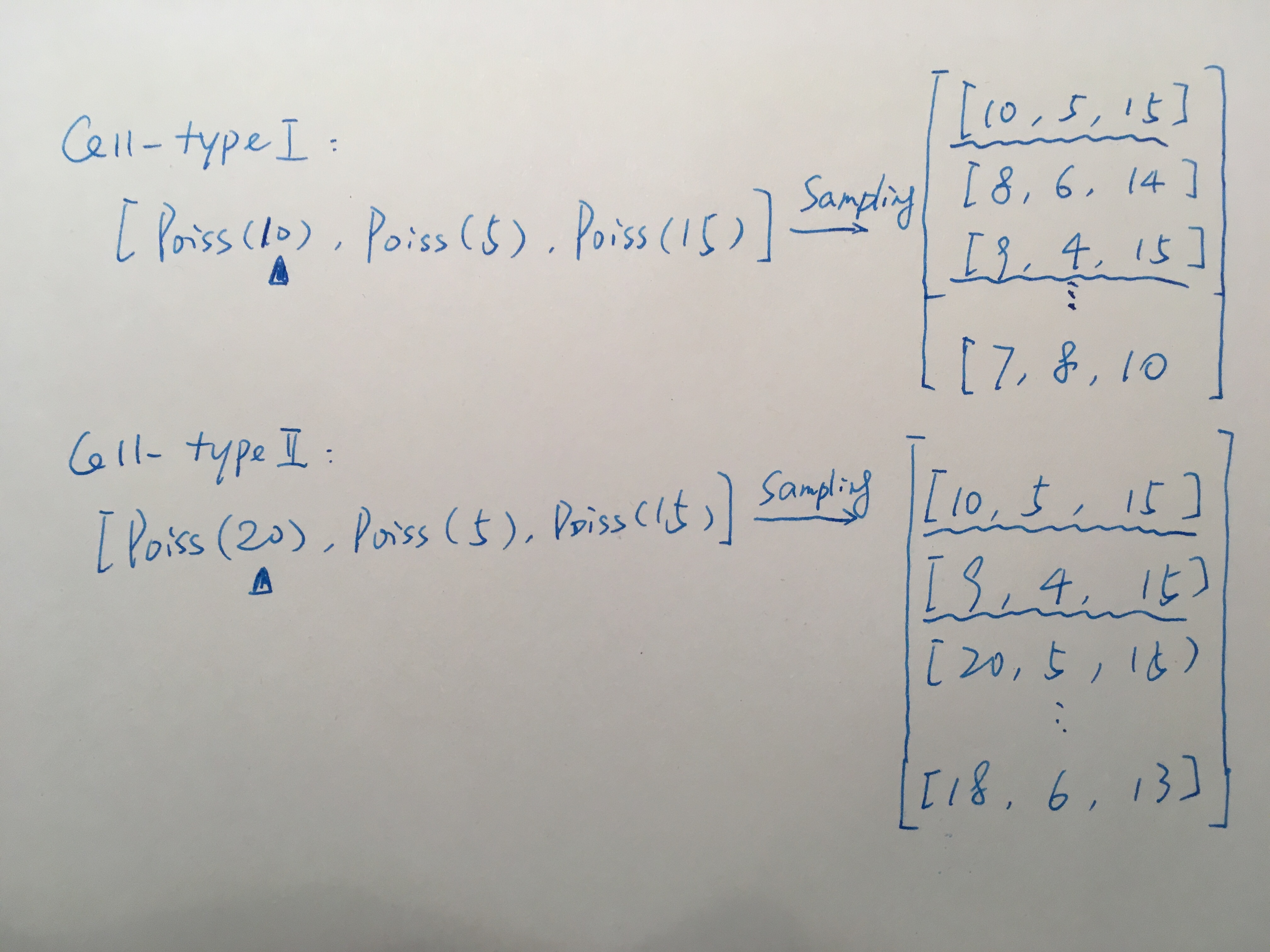
idx_hig <- (num_genes/3*2 + 1) : num_genesObserved cells () are sampled from the profile. Each gene follows its Poisson distribution where . This is consistent to the UMI-filtered single-cell RNA-seq data when the pure RNA spike-ins are the loading input.
num_cells <- 500
# a matrix with cells x genes
mat_apple <- round(sapply(expect_apple,
                          function(e) rpois(n = num_cells, lambda = e)))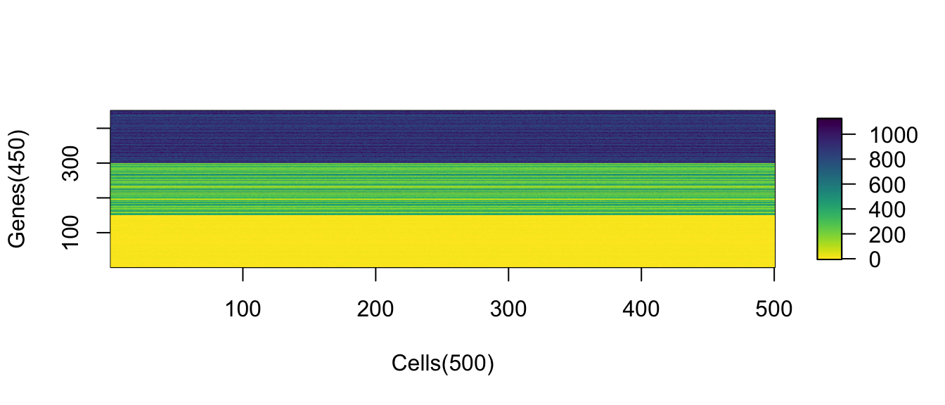
(#fig:viz_expr_mat)Observed expression matrix with cells on rows and genes on columns
Create “A” and “B”
In order to create new cell type “A” and “B”, each of them has ~40 genes being upregulated. There situations were investigated:
num_up_genes <- round((num_genes/3) / 4)- low-expressed genes: () adding
- medium-expressed genes: () adding
- high-expressed genes: () adding
All the add-ups roughly take half of the expression.
Low
idx_up_1 <- head(idx_low, num_up_genes)
idx_up_2 <- tail(idx_low, num_up_genes)
expect_banana <- expect_apple
expect_banana[idx_up_1] <- expect_banana[idx_up_1] + runif(n=num_up_genes,
min=4, max=10)
mat_banana <- round(sapply(expect_banana,
function(e) rpois(n = num_cells, lambda = e)))
expect_cherry <- expect_apple
expect_cherry[idx_up_2] <- expect_cherry[idx_up_2] + runif(n=num_up_genes,
min=4, max=10)
mat_cherry <- round(sapply(expect_cherry,
function(e) rpois(n = num_cells, lambda = e)))Bonus: Create “AB”
expect_guava <- expect_apple
idx_down <- idx_up_2
num_down_genes <- num_up_genes
# upregulated genes
expect_guava[idx_up_1] <- expect_guava[idx_up_1] +
runif(n=num_up_genes, min=4* sqrt(2)/2, max=10*sqrt(2)/2)
# downregulated genes
num_down_genes <- num_up_genes
expect_guava[idx_down] <- expect_guava[idx_down] -
runif(n=num_down_genes, min=4*sqrt(2)/2, max=10*sqrt(2)/2)
expect_guava[expect_guava < 0] <- 0
mat_guava <- round(sapply(expect_guava,
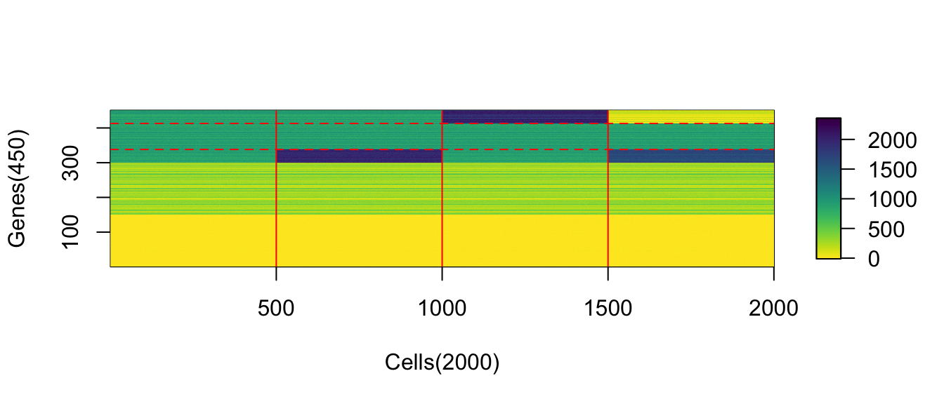
function(e) rpois(n = num_cells, lambda = e)))Visualize the expression profile and the sampled cells
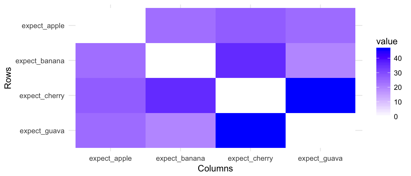
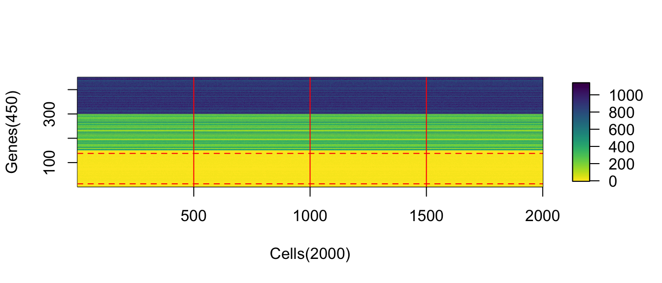
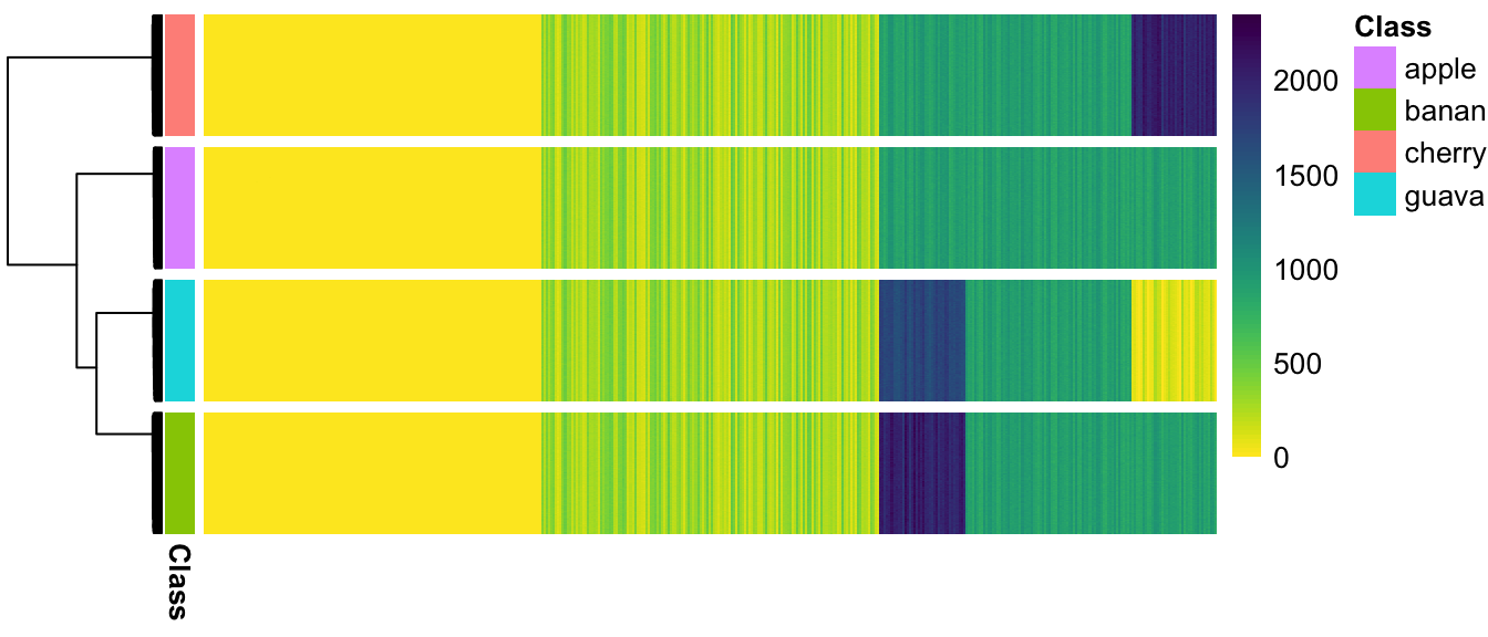
(#fig:image_matrix_ChangeLow)The absolute values of upregulation for low-expressed genes is not obvious
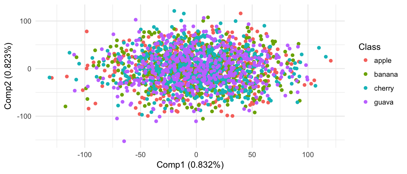
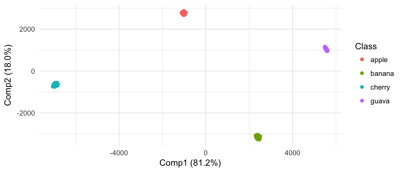
From results of clustering and projection down to 2D PCA space, the different populatons are not considered as different.
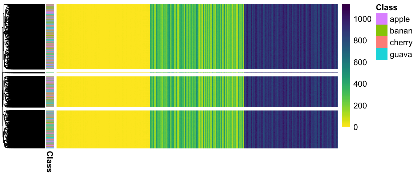
(#fig:pheatmap_allcells_ChangeLow)Populations are not separated at all
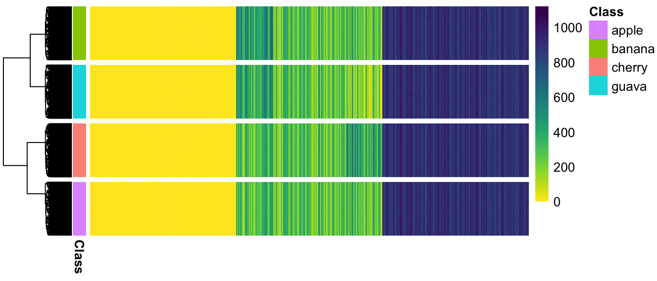
Med
Similar procedure is performed again to upregulate med-expressed genes and do sampling cells from expression profile.
Visualize expression matrix of the sample cells
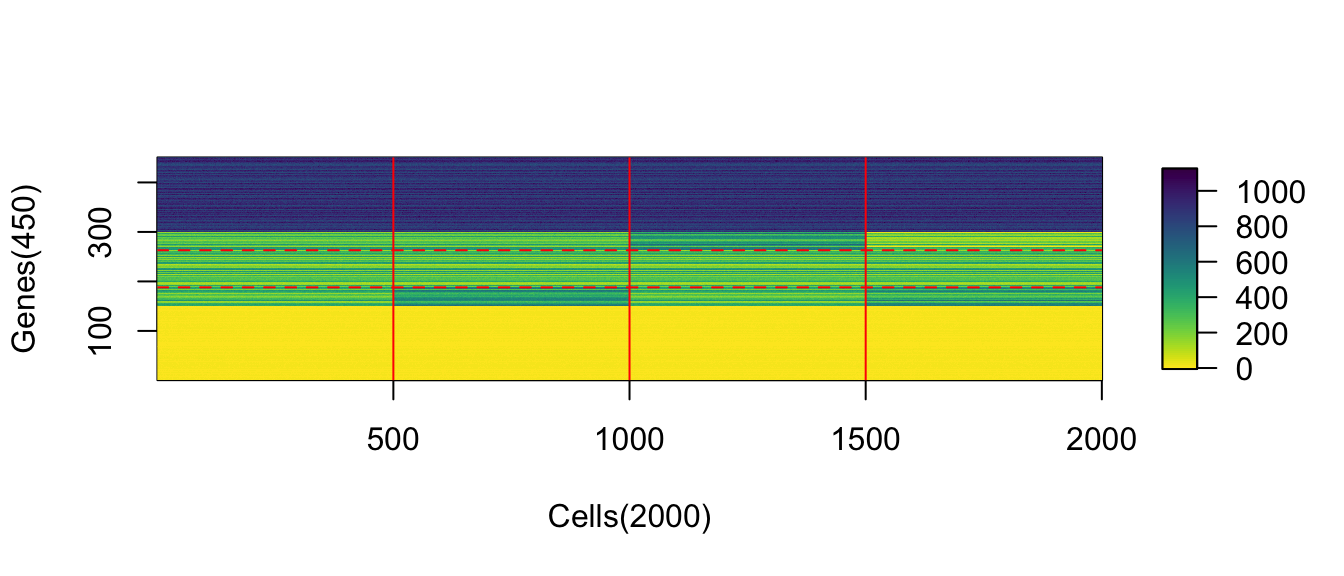
(#fig:image_matrix_ChangeMed)The absolute value of upregulation of med-expressed genes could be observed.
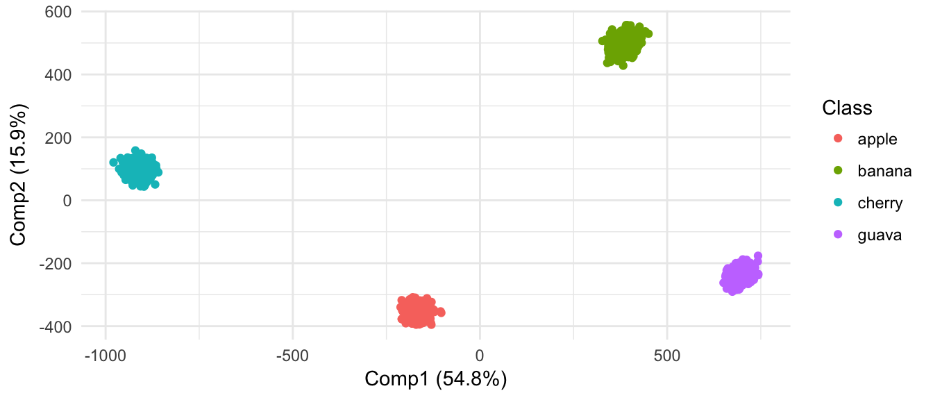
Populations are detected.
High
Not surprisingly, populations are found.
Summary
I did not make a good example to hack distance, but re-learned the following messages:
- Highly expressed genes (with high variance) have more weights when counting the sample distance, which implied the need of variance stablization.
Possible to follow-up:
- Gene-wise normalize
- Focus on low-expressed genes